Posey's Tips & Tricks
Working With Checkboxes in Excel, Part 2: Adding Complexity
Here's how to build smarter checklists in Excel using checkboxes, conditional formatting and task dependencies to help with multi-step processes.
In my previous article in this series, I walked you through the process of setting up a really simple checklist in which selecting a checkbox causes a checklist item to become marked out. As I wrote that particular piece, I began to wonder about more complex checklists in which there is a dependency relationship between tasks. In other words, certain tasks cannot be started until other tasks are complete.
My original idea was to gray out any tasks that could not be started until another task is finished and then activate those tasks when the prerequisites have been met. Unfortunately, Excel checkboxes do not directly support this type of behavior. Remember, you can use a checkbox to launch a macro or to format a cell's text, but those seem to be the only options. Even so, I have figured out a roundabout method for building a task list in which some tasks are dependent on others.
For the purposes of this article, I will be creating a spreadsheet that acts as an employee onboarding template. The reason why I am using this particular example is because when it comes to employee onboarding, there are certain tasks that usually have to be completed in a particular order. As an example, it might be difficult to schedule a goal planning meeting with the employee's manager until the employee has access to an Outlook calendar and the employee can't get access to Outlook until an account has been set up.
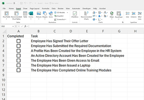
In my example spreadsheet, the first column will contain the task description and the second column will contain the corresponding checkboxes. You can see what my basic spreadsheet looks like in Figure 1.
 [Click on image for larger view.]
Figure 1. This is my employee onboarding spreadsheet.
[Click on image for larger view.]
Figure 1. This is my employee onboarding spreadsheet.
As before, the first thing that needs to be done in order to make this checklist functional is to pick a column (preferably offscreen) that will store the checkbox state. I will be using column N, so that the value of the checkbox residing at A2 will be displayed at N2, the value of the A3 checkbox will be displayed at N3, and so on. To create this relationship between a checkbox and a cell, right click on the checkbox and select the Format Control option from the shortcut menu. When prompted, enter the cell that will be used to store the checkbox's value and click OK.
The next step in the process is to figure out which of the tasks on the lists are top level tasks. In other words, which tasks can be completed without there being a dependency on any other tasks. Select all of the tasks except for the top-level tasks that you have identified and set the text color to light gray. You can do this by going to the Home tab and setting the font color.
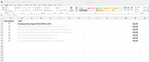
In my sample employee onboarding form, the first step in the onboarding process is that the employee has to sign their offer letter. Nothing else can happen until the offer has been signed. Therefore, I left the text color for this step set to black, and I colored the rest of the text gray, making it appear as though the option is grayed out, even though it isn't. You can see what this looks like in Figure 2.
 [Click on image for larger view.]
Figure 2. I have made it look as though all but the first option is grayed out
[Click on image for larger view.]
Figure 2. I have made it look as though all but the first option is grayed out
The next task that would need to be completed as a part of the employee onboarding process is that the employee has submitted the required documentation. After all, that would need to happen before the employee could be set up in the HR system or issues an Active Directory account. Therefore, let's make it so that when the checkbox is selected indicating that the employee has signed their offer letter, that task is crossed off the list and the option to submit documentation is no longer grayed out.
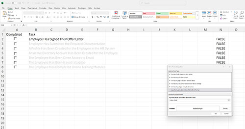
Crossing an item off the list works in exactly the same way as what I discussed in the first article. In this case, we would select the Employee Has Signed Their Offer Letter option, click on Conditional Formatting, and create a new rule that will apply the strikethrough style of the value shown in N2 is True. You can see what this looks like in Figure 3.
 [Click on image for larger view.]
Figure 3. I have created a formatting rule to strike through the text of a completed list item.
[Click on image for larger view.]
Figure 3. I have created a formatting rule to strike through the text of a completed list item.
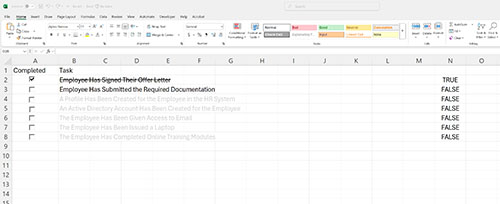
The next step is to select the next task on the list (Employee Has Submitted the Required Documentation) and create a conditional formatting rule. We are going to point the new rule at cell N2, just like before. Remember, if cell N2 is set to True then it means that the previous task has been completed. The difference is that this time, rather than clicking on the Format button and selecting the strikethrough style, we are going to click on the Color dropdown and set the color to black. This way, when the previous task is completed, the text will no longer appear to be grayed out. You can see the effect in Figure 4.
 [Click on image for larger view.]
Figure 4. A task has been completed and the next task is now available.
[Click on image for larger view.]
Figure 4. A task has been completed and the next task is now available.
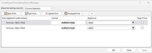
So what about a third tier task? Well, my second tier task were to be completed, then there are multiple third tier tasks that could be made available. I would simply need to create a conditional formatting rule for each. But remember, the second task (Employee Has Submitted the Required Documentation) already has a rule associated with it. Fortunately, Excel will allow you to associate multiple conditional formatting rules with a cell. If you look at Figure 5 for example, you can see that there is a rule to apply the strikethrough and another rule to change the text color.
 [Click on image for larger view.]
Figure 5. A cell can contain multiple conditional formatting rules.
[Click on image for larger view.]
Figure 5. A cell can contain multiple conditional formatting rules.
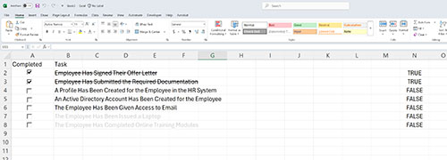
You can also create multiple conditional formatting rules that look at the value contained within a single cell. If you look at Figure 6, you can see that the first two tasks on my list have been completed. With the second task complete, multiple third tier tasks are now available to be performed. All three of these tasks are based on the value of cell N3.
 [Click on image for larger view.]
Figure 6. The third tier tasks are now activated.
[Click on image for larger view.]
Figure 6. The third tier tasks are now activated.
About the Author
Brien Posey is a 22-time Microsoft MVP with decades of IT experience. As a freelance writer, Posey has written thousands of articles and contributed to several dozen books on a wide variety of IT topics. Prior to going freelance, Posey was a CIO for a national chain of hospitals and health care facilities. He has also served as a network administrator for some of the country's largest insurance companies and for the Department of Defense at Fort Knox. In addition to his continued work in IT, Posey has spent the last several years actively training as a commercial scientist-astronaut candidate in preparation to fly on a mission to study polar mesospheric clouds from space. You can follow his spaceflight training on his Web site.