Posey's Tips & Tricks
Working With Checkboxes in Excel, Part 1: Adding and Configuring
Learn how to add, configure and use checkboxes in Excel to create interactive task lists and trigger formatting without relying on macros.
Recently, Microsoft has introduced the ability to add checkboxes to Excel spreadsheets. These checkboxes can be super convenient for cases in which you want to build automation into a spreadsheet. As an example, you might use a checkbox as a mechanism for activating a macro. But even if your company does not allow the use of macros, Excel checkboxes can be useful for automatically formatting a spreadsheet. Imagine for instance, that you create a task list within Excel. You could make it so that when you mark an item as done (by selecting a checkbox), the corresponding item is automatically marked off the list.
As useful as checkboxes might be in Excel, they aren't completely intuitive. As such, I wanted to write a two-part series on how to use checkboxes. In this first part of the series, I will show you how to add a checkbox to a spreadsheet and I will walk you through some of the basics of configuring a checkbox to do whatever it is that you want it to do. In part two, I will walk you through the process of setting up a somewhat advanced use case.
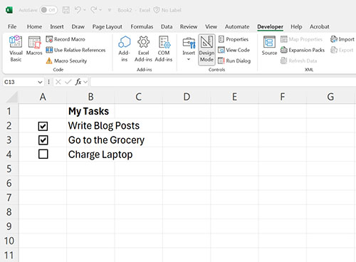
Before you can add checkboxes to an Excel worksheet, you will need to expose the Developer tab (if it is not already visible). To do so, click on the File menu and then select Options, followed by Customize Ribbon. Select the Developer checkbox from the pane on the right, as shown in Figure 1. Click OK to add the Developer tab to the Excel GUI interface.
 [Click on image for larger view.]
Figure 1. Select the Developer checkbox and click OK.
[Click on image for larger view.]
Figure 1. Select the Developer checkbox and click OK.
To add a checkbox to a spreadsheet, you will need only to go to the Developer tab, click on the Insert option and then click on the checkbox icon.
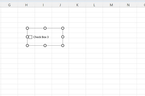
Interestingly, when you add a checkbox to an Excel spreadsheet, the checkbox is not inserted into a cell. Instead, the checkbox is added as a graphical item, over top of the spreadsheet. If you have ever inserted an object into a Microsoft Publisher document, the process is almost identical to that of adding a checkbox to an Excel spreadsheet. You can see what this process looks like in Figure 2.
 [Click on image for larger view.]
Figure 2. Excel checkboxes are added as graphical objects and are not bound to a cell.
[Click on image for larger view.]
Figure 2. Excel checkboxes are added as graphical objects and are not bound to a cell.
Even though checkboxes are not tied to a specific cell, you can easily resize or reposition a checkbox. To do so, right click on the checkbox and then use the dots shown in the previous figure to size the checkbox according to your needs. You can also move the mouse pointer to the middle of the checkbox and then click and drag the checkbox to the desired position.
If you look back at the previous figure, you will notice that the words Checkbox 3 appear just to the right of the checkbox. That's fine if you are just experimenting with checkboxes and trying to get a feel for how they work, but if you are trying to add a checkbox to a spreadsheet that you actually plan on using for something then you will probably want to delete or replace this text. My personal preference is to store text in cells rather than binding the text to the checkbox object, but either option works.
To remove or replace the text that appears next to a checkbox, Right click on the checkbox object and then select the Edit Text command from the shortcut menu. This causes Excel to place a cursor within the text block, allowing you to delete or type over the existing text.
So now that I have introduced a few basic concepts, I want to walk you through setting up a really simple use case. We will set up a checklist and make it so that items are marked off a list when completed.
To get started, create a new spreadsheet and place a few checklist items in column B. Those items can be anything. Now, create a checkbox for each of your checklist items and place the checkboxes over column A. You can see an example of this in Figure 3. As you create the checkboxes, be sure to size them to match the height of the row. Otherwise, the checkboxes may overlap and interfere with one another.
 [Click on image for larger view.]
Figure 3. Create a simple task list and create a checkbox for each item.
[Click on image for larger view.]
Figure 3. Create a simple task list and create a checkbox for each item.
The next thing that you will need is a cell to store each checkbox's state. You will probably want to choose a column that appears outside of the visible part of the spreadsheet. Now, right click on the first of your checkboxes and select the Format Control option from the shortcut menu. When the Format Control dialog box appears, select the Control tab and then enter the location of the cell that will store the checkbox's value. In my case, I am going to use cell N2 to store the value of the checkbox that resides at A2. Hence, I would enter N2 into the Cell Link field and click OK. You will need to repeat this process for each checkbox. In the end, you should have a column that reflects a status of TRUE or FALSE depending on whether or not a checkbox is selected. You may occasionally have to click a checkbox a couple of times before the status will show up. You can see what this looks like in Figure 4.
 [Click on image for larger view.]
Figure 4. Column N reflects the checkbox status.
[Click on image for larger view.]
Figure 4. Column N reflects the checkbox status.
Now, select a checklist item (the text, not the checkbox) and then go to the Home tab and click on the Conditional Formatting icon. When prompted, choose the New Rule option.
When prompted, select the Use a Formula to Determine Which Cells to Format option. The formula must look at the corresponding checkbox's value to determine whether it is TRUE or FALSE. As an example, the status for the first item on my checklist is stored in cell N2. Hence, the formula would be =$N2=TRUE. Now, click the Format button, select the Strikethrough option and click OK. Make sure that the preview shows sample text being marked through, as shown in Figure 5. Click OK again to complete the process. Now, repeat this process for any remaining checkboxes. When you are done, you can strike through list items by selecting their checkboxes, as shown in Figure 6.
 [Click on image for larger view.]
Figure 5. Make sure that the preview text uses the strikethrough effect.
[Click on image for larger view.]
Figure 5. Make sure that the preview text uses the strikethrough effect.
 [Click on image for larger view.]
Figure 6. This is what the completed spreadsheet looks like.
[Click on image for larger view.]
Figure 6. This is what the completed spreadsheet looks like.
Now that I have walked you through a simple example of how to use checkboxes in Excel, I want to show you a slightly more advanced technique in Part 2 of this series.
About the Author
Brien Posey is a 22-time Microsoft MVP with decades of IT experience. As a freelance writer, Posey has written thousands of articles and contributed to several dozen books on a wide variety of IT topics. Prior to going freelance, Posey was a CIO for a national chain of hospitals and health care facilities. He has also served as a network administrator for some of the country's largest insurance companies and for the Department of Defense at Fort Knox. In addition to his continued work in IT, Posey has spent the last several years actively training as a commercial scientist-astronaut candidate in preparation to fly on a mission to study polar mesospheric clouds from space. You can follow his spaceflight training on his Web site.