Posey's Tips & Tricks
How To Use Microsoft Office for Asset Management, Part 3
Working with absolute and relative cell references in Excel, plus retrieving a value from a second sheet.
At the conclusion of Part 2, I showed you a screen capture of a spreadsheet in which I looked up values from elsewhere in the spreadsheet. Some of these values were retrieved without issue, but others produced errors, as shown in Figure 1 below. So what's going on?
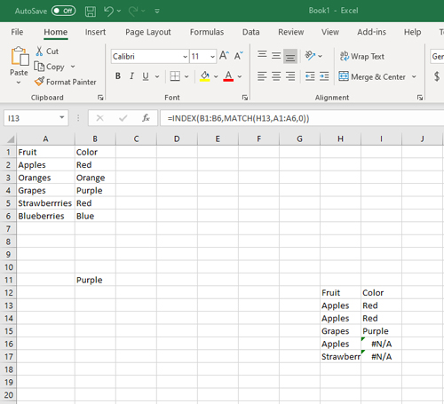 Figure 1: Some of the cells are displaying errors.
The problem occurred because I used relative references instead of absolute references. Notice in Figure 1 that the index portion of the formula references cells B1 through B6. When I copy the formula and paste it into the cell beneath the one that is currently selected, the index points to B2 through B7. If I paste it to the next cell on the list, the index for that cell points to B3 to B8.
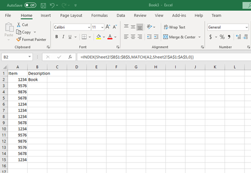
The relative reference to the cell range of B1 through B6 is expressed as B1:B6. If I wanted to change this to an absolute reference, I would simply need to reformat the range as $B$1:$B$6. In the formula that I used earlier, I also need to change the A1 to A6 reference to an absolute reference. You can see the new formula in Figure 2. Notice that when I copy this formula to the remaining cells, the results all display correctly.
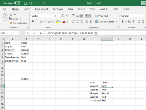 [Click on image for larger view.] Figure 2: I changed some of the relative references to absolute references.
Now that I have shown you the difference between relative and absolute references, let's address the last piece of the puzzle, which involves retrieving a value from another sheet. In Excel, you can reference a cell or a range from another sheet by typing the sheet name, followed by an exclamation point and the cell or range that you want to reference. For example, if I wanted to reference the A1:A10 range within Sheet 2, I would enter it as Sheet2!A1:A10.
Let's get back to the task at hand. As you may recall from the previous column, I created an Excel document consisting of two sheets. Sheet 1 contains a list of item numbers. We will pretend that these item numbers have been scanned in using a barcode reader. There is an empty column for item descriptions, as shown in Figure 3.
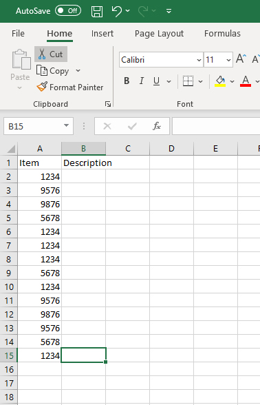 Figure 3: This is my inventory sheet.
Sheet 2 of the document is my catalog. It contains item numbers and a description of each item, as shown in Figure 4. Sheet 1 will reference this catalog to figure out the name of each item based on its item number.
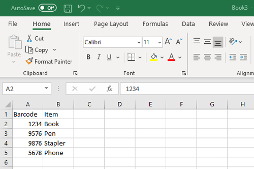 Figure 4: This is my catalog.
If you look at Figure 5, you can see that the formula I am using is almost identical to the one used in the previous spreadsheet. The biggest difference is that I am making references to Sheet 2 as opposed to everything being on the same sheet.
 [Click on image for larger view.] Figure 5: The formula that I am using is very similar to the one used previously.
If I copy the formula and paste it into the remaining cells in the B column, the spreadsheet displays the names of all of my inventory items, as shown in Figure 6.
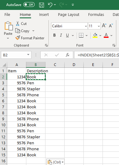 Figure 6: The spreadsheet has been fully populated.
Obviously, a production inventory-tracking system (even one used by the smallest businesses) needs more functionality than what I have shown here. This is just a starting point. There are any number of ways that you could improve this process. One idea might be to add some extra fields to the catalog such as size, weight, color or that sort of thing.
Another option might be to tally the results. You can do this by selecting the items and then clicking on the Sort A to Z button on the toolbar. Once the items have been sorted, select the Description column (be sure to select the column header, too). Now select the Data tab and then click on the Subtotal button found on the toolbar. This will cause Excel to open the Subtotal dialog box. This dialog box includes a drop-down called Use Functions. By default, this is set to Sum, but you will need to change it to Count, as shown in Figure 7.
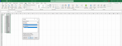 [Click on image for larger view.] Figure 7: Set the Use Function option to count.
Now, click OK and Excel will provide you with a count of each of the items that you scanned. You can see the end result in Figure 8.
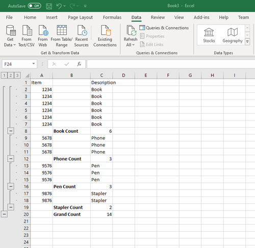 [Click on image for larger view.] Figure 8: Excel has produced a count of my inventory items.
About the Author
Brien Posey is a 22-time Microsoft MVP with decades of IT experience. As a freelance writer, Posey has written thousands of articles and contributed to several dozen books on a wide variety of IT topics. Prior to going freelance, Posey was a CIO for a national chain of hospitals and health care facilities. He has also served as a network administrator for some of the country's largest insurance companies and for the Department of Defense at Fort Knox. In addition to his continued work in IT, Posey has spent the last several years actively training as a commercial scientist-astronaut candidate in preparation to fly on a mission to study polar mesospheric clouds from space. You can follow his spaceflight training on his Web site.