Posey's Tips & Tricks
Simplifying the Process of Working with Large Excel Spreadsheets
Here are a few tips that will improve your efficiency and get you out of that massive data spreadsheet as soon as possible.
About a month ago, I wrapped up a massive data reorganization project. The particulars of this project aren't important because they are unique to my own environment. However, the nature of the project resulted in me having to create a massive spreadsheet containing thousands of populated cells. As I worked through the project, I continually had to refer to various cells scattered throughout the spreadsheet. Unfortunately, automation just wasn't an option and there was really no alternative to manually reviewing the data. As you can imagine, this was a super tedious and time consuming project, and I am glad that it's over.
One of the things that made this project so challenging was that in spite of me having multiple large format monitors attached to my PC, the sheer size of the spreadsheet meant that it was impossible to view the data all at once. As such, I used a few different techniques to make the spreadsheet easier to use.
Header Locking
When I began to realize just how large the spreadsheet was going to be, one of the first things that I did was to lock the header rows. Doing so makes it so that the headers (columns headers and / or row headers) do not move as you scroll through the spreadsheet. Locking the header rows made it way easier to keep track of what I was looking at during the review process.
Excel refers to the process of locking a row or a column as freezing. To freeze a header row, click on the View tab and then click on the Freeze Panes icon. As you can see in Figure 1, Excel provides you with three options. You can freeze the top row, you can freeze the first column, or you can freeze panes.
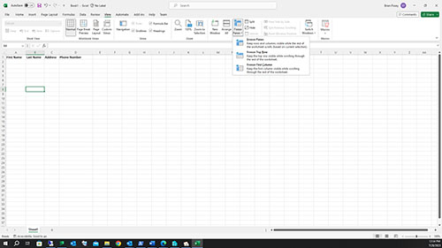 [Click on image for larger view.] Figure 1. Excel gives you three different options for freezing headers in your spreadsheet.
The options to freeze the top row or the first column are self-explanatory. The Freeze Panes option is intended for use in more complex situations in which you need to freeze multiple rows or columns. To use this option, just select the row that is just below the row that you want to freeze. As an alternative, you could also select the column just to the right of the one that you want to freeze. When you have made your selection, select the Freeze Pane option. Everything above or to the left of your selection (depending on whether you selected a row or a column) will be frozen and will remain on screen as you scroll through the spreadsheet. Incidentally, if you make a mistake, you can undo the operation by going back to the Freeze Panes icon and selecting the unfreeze option.
Splitting a Spreadsheet into Multiple Panes
Another technique that I found useful when working with my massive spreadsheet was to split the sheet into multiple panes. Doing so allows you to have two different areas of the same spreadsheet on the screen simultaneously.
This technique works somewhat similarly to the technique used for freezing header rows, except that it is designed to allow you to work in two different sections of the sheet at the same time. To split a sheet into two panes, Select the row below the point where you want the split to occur or select the column just to the right of the split point. Next, select the View tab and click on the split icon, which you can see in Figure 2.
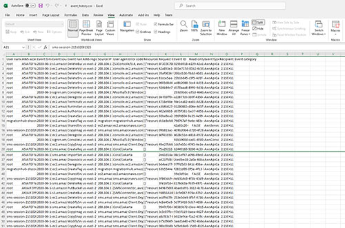 [Click on image for larger view.] Figure 2. Click on the Split icon to split the sheet into two.
As you can see in the figure, Excel places a dividing line at the split point. If you look at the far right side of the figure, you will notice that there are now two scroll bars, meaning that you can scroll the two sections independently of one another.
Viewing Multiple Tabs at the Same Time
One last trick that I wanted to mention is that if your workbook (the excel document) contains multiple spreadsheets and you have multiple monitors, you can view each sheet on a separate monitor so that you don't have to constantly switch back and forth between sheets.
To do so, begin by opening your Excel document as you normally would and then select the document's primary worksheet (which ever worksheet you will be using most often). Next, select the View tab, and then click the New Window button. This will cause Windows to open a secondary window containing a copy of your spreadsheet. Now simply drag this secondary window to another monitor and then click on the tab corresponding to the sheet that you want to view on that monitor. If you have more than two sheets, you can open additional windows.
About the Author
Brien Posey is a 22-time Microsoft MVP with decades of IT experience. As a freelance writer, Posey has written thousands of articles and contributed to several dozen books on a wide variety of IT topics. Prior to going freelance, Posey was a CIO for a national chain of hospitals and health care facilities. He has also served as a network administrator for some of the country's largest insurance companies and for the Department of Defense at Fort Knox. In addition to his continued work in IT, Posey has spent the last several years actively training as a commercial scientist-astronaut candidate in preparation to fly on a mission to study polar mesospheric clouds from space. You can follow his spaceflight training on his Web site.