Posey's Tips & Tricks
Using Functions To Alter the Appearance of an Excel Spreadsheet
Recently, I have been doing quite a bit of work involving the use of functions inside Excel spreadsheets. Although functions are probably most often used for computational purposes, functions can also be used for changing a spreadsheet's overall appearance.
One of the functions that I have been spending quite a bit of time with lately is the MOD function. In case you aren't familiar with this function, its purpose is to determine the remainder when one number is divided by another. For example, if you were to divide the number 7 by 3, the remainder would be equal to 1.
To use the MOD function, we have to supply two numbers -- a numerator and a denominator. For those whose math skills might be a bit rusty, a fraction is essentially a way of representing a division operation. The number on top is called the numerator and the number on the bottom of the fraction is the denominator. The numerator is divided by the denominator.
Hence, the previous example of 7 divided by 3 could be expressed as an improper fraction of 7/3. When evaluated, the answer to this expression is two and one-third, which can also be expressed as 2.333, or two with a remainder of 1. It is this remainder of 1 that would be returned by the MOD function.
So to make things just a little bit more clear, let's take a look at Excel and see how the MOD function works. Here is the syntax:
=MOD(numerator, denominator)
If I were to plug the numerator (7) and the denominator (3) from my previous example into this function, it would look like this:
=MOD(7,3)
As you can see in Figure 1, this function returns a value of 1, which is the remainder when 7 is divided by 3.
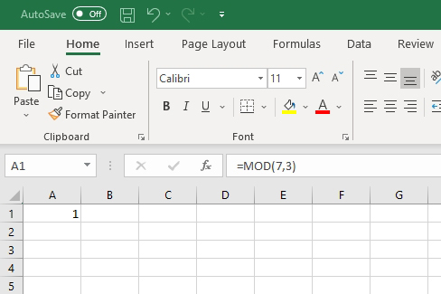 Figure 1: The function =MOD(7,3) returns a value of 1.
OK, so the MOD function returns the remainder of a division operation. That's all well and good, but as you may recall, I suggested that this function could actually be used to format the appearance of an Excel worksheet.
In Excel, functions aren't used solely to compute values within the sheet. Excel includes a feature called Conditional Formatting, and this feature allows you to use a function to determine how a spreadsheet should be formatted.
Let's suppose for a moment that I wanted to apply shading to every other row of a spreadsheet. There are a few different ways to accomplish this, but let's use the MOD function. Begin by selecting either the entire sheet or the portion of the sheet that you want to format. Next, click on the Conditional Formatting icon found in the toolbar. Next, choose the New Rule option from the Conditional Formatting menu.
At this point, Excel displays the New Formatting Rule dialog box. As you can see in Figure 2, this dialog box includes an option to use a formula to control which cells will be formatted. With this option selected, the only things left to do are to specify the formula and the desired format.
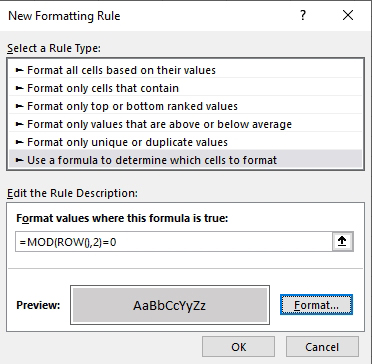 Figure 2: This is how you apply conditional formatting using a function.
If the goal is to shade every other line, then the formula that you can use is:
=MOD(ROW(),2)=0
Before I show you how this works, I want to give credit where credit is due: Microsoft lists this formula on one of the Office support pages, so I did not come up with the formula on my own.
So let's take a look at how the formula works. You are already familiar with the =MOD portion of the formula. However, this formula looks a little bit different from what you saw in my previous examples. Rather than us specifying a numerator and a denominator, the numerator is replaced by ROW, indicating that we are working with individual rows. The only numerical value specified within the parentheses is 2. There is also an equal sign and a 0 following the formula.
This formula checks if a row number is evenly divisible by 2. In other words, the row number becomes the numerator and 2 is the denominator. If the remainder is 0 (which will only be the case for evenly numbered rows), then the conditional formatting is applied.
Choosing the formatting type is simply a matter of clicking the Format button shown in Figure 2 above. This opens a dialog box that lets you choose anything from fonts to fill colors. If you look back at Figure 2, you can see that I have chosen a grey fill color.
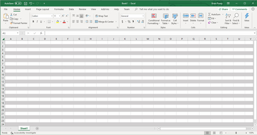 [Click on image for larger view.] Figure 3: The spreadsheet has been formatted according to the specified formula.
Upon clicking OK, the spreadsheet is formatted with my chosen fill color on every other line, as shown in Figure 3. It's that easy.
About the Author
Brien Posey is a 22-time Microsoft MVP with decades of IT experience. As a freelance writer, Posey has written thousands of articles and contributed to several dozen books on a wide variety of IT topics. Prior to going freelance, Posey was a CIO for a national chain of hospitals and health care facilities. He has also served as a network administrator for some of the country's largest insurance companies and for the Department of Defense at Fort Knox. In addition to his continued work in IT, Posey has spent the last several years actively training as a commercial scientist-astronaut candidate in preparation to fly on a mission to study polar mesospheric clouds from space. You can follow his spaceflight training on his Web site.